Using Deep Learning Tools
들어가기에 앞서
지난 시간에 CNN에 대해 간략하게 나마 알아보았다.
이번에는 교수님께서 제공해주신 예제들을 통해 친숙해져보도록 하겠다.
!nvidia-smi는 nvidia gpu resource들을 모니터링하는 명령어이다.
1 | !nvidia-smi |
Wed Jan 20 05:13:24 2021
+-----------------------------------------------------------------------------+
| NVIDIA-SMI 410.104      Driver Version: 410.104      CUDA Version: 10.1     |
|-------------------------------+----------------------+----------------------+
| GPU  Name        Persistence-M| Bus-Id        Disp.A | Volatile Uncorr. ECC |
| Fan  Temp  Perf  Pwr:Usage/Cap|         Memory-Usage | GPU-Util  Compute M. |
|===============================+======================+======================|
|   0  Tesla V100-DGXS...  On   | 00000000:07:00.0 Off |                    0 |
| N/A   41C    P0    51W / 300W |   1561MiB / 32478MiB |      0%      Default |
+-------------------------------+----------------------+----------------------+
|   1  Tesla V100-DGXS...  On   | 00000000:08:00.0 Off |                    0 |
| N/A   40C    P0    54W / 300W |    626MiB / 32478MiB |      0%      Default |
+-------------------------------+----------------------+----------------------+
|   2  Tesla V100-DGXS...  On   | 00000000:0E:00.0 Off |                    0 |
| N/A   40C    P0    50W / 300W |  27829MiB / 32478MiB |      0%      Default |
+-------------------------------+----------------------+----------------------+
|   3  Tesla V100-DGXS...  On   | 00000000:0F:00.0 Off |                    0 |
| N/A   40C    P0    49W / 300W |    652MiB / 32478MiB |      0%      Default |
+-------------------------------+----------------------+----------------------+

+-----------------------------------------------------------------------------+
| Processes:                                                       GPU Memory |
|  GPU       PID   Type   Process name                             Usage      |
|=============================================================================|
+-----------------------------------------------------------------------------+
랩실에서 실제로 사용하고 있는 서버이기 때문에 리소스를 확인하고 적절히 분배해서 사용해야한다.
1 | # using gpu:/1 |
위와 같은 코드를 사용하면 GPU #1번을 사용하는 것이다. 또한, 한꺼번에 모든 메모리를 사용하는 것이 아닌 tf.config.experimental.set_memory_growth를 사용해 메모리를 증가시키며 사용한다.
1 | # using gpu:/1 |
MNIST dataset은 튜링어워드를 수상하셨던 Convolution network의 창시자 Yann LeCun가 제공해주시는 데이터셋이다.
이를 활용하여 실습을 진행해보겠다.
MNIST dataset은 손으로 쓴 숫자 이미지를 벡터로 나타낸 images와 그 이미지가 의미하는 숫자를 나타내는 labels로 이루어져 있다. 한개의 이미지는 28*28(=784)의 픽셀로 이루어져 있기 때문에 이는 784차원의 벡터로 저장되어 있고 진하기의 정도에 따라 0~1사이의 값이 들어있다. 예시는 다음과 같다.

1 | from tensorflow.keras.datasets import mnist |
# of train data :  (60000, 28, 28)
# of test data :  (10000, 28, 28)
1 | plt.imshow(x_train[509], cmap='gray') |
<matplotlib.image.AxesImage at 0x7f14e8b00940>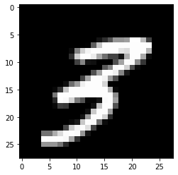
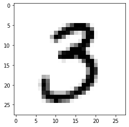
우선 CNN을 적용시키기 이전에 데이터를 vectorization시킨 후 진행해보겠다.
1 | # Vectorization for ANN |
1 | model = Sequential() |
Model: "sequential"
_________________________________________________________________
Layer (type)                 Output Shape              Param #
=================================================================
dense (Dense)                (None, 512)               401920
_________________________________________________________________
dense_1 (Dense)              (None, 512)               262656
_________________________________________________________________
dense_2 (Dense)              (None, 10)                5130
=================================================================
Total params: 669,706
Trainable params: 669,706
Non-trainable params: 0
_________________________________________________________________
1 | model.compile(loss='categorical_crossentropy', metrics=['accuracy']) |
Epoch 1/20
1875/1875 [==============================] - 6s 3ms/step - loss: 0.3957 - accuracy: 0.9521 - val_loss: 0.5461 - val_accuracy: 0.9337
Epoch 2/20
1875/1875 [==============================] - 6s 3ms/step - loss: 0.3798 - accuracy: 0.9524 - val_loss: 0.7209 - val_accuracy: 0.9506
Epoch 3/20
1875/1875 [==============================] - 6s 3ms/step - loss: 0.3913 - accuracy: 0.9522 - val_loss: 0.5986 - val_accuracy: 0.9464
Epoch 4/20
1875/1875 [==============================] - 6s 3ms/step - loss: 0.3965 - accuracy: 0.9505 - val_loss: 0.6736 - val_accuracy: 0.9391
Epoch 5/20
1875/1875 [==============================] - 6s 3ms/step - loss: 0.4349 - accuracy: 0.9540 - val_loss: 0.7524 - val_accuracy: 0.9441
Epoch 6/20
1875/1875 [==============================] - 6s 3ms/step - loss: 0.4307 - accuracy: 0.9506 - val_loss: 0.9400 - val_accuracy: 0.9461
Epoch 7/20
1875/1875 [==============================] - 6s 3ms/step - loss: 0.4567 - accuracy: 0.9509 - val_loss: 0.8693 - val_accuracy: 0.9406
Epoch 8/20
1875/1875 [==============================] - 6s 3ms/step - loss: 0.4598 - accuracy: 0.9475 - val_loss: 0.9901 - val_accuracy: 0.9225
Epoch 9/20
1875/1875 [==============================] - 6s 3ms/step - loss: 0.4730 - accuracy: 0.9471 - val_loss: 1.5888 - val_accuracy: 0.9191
Epoch 10/20
1875/1875 [==============================] - 6s 3ms/step - loss: 0.4903 - accuracy: 0.9363 - val_loss: 0.9527 - val_accuracy: 0.9295
Epoch 11/20
1875/1875 [==============================] - 6s 3ms/step - loss: 0.5425 - accuracy: 0.9351 - val_loss: 1.4321 - val_accuracy: 0.9451
Epoch 12/20
1875/1875 [==============================] - 6s 3ms/step - loss: 0.5320 - accuracy: 0.9397 - val_loss: 1.7940 - val_accuracy: 0.9428
Epoch 13/20
1875/1875 [==============================] - 6s 3ms/step - loss: 0.5362 - accuracy: 0.9346 - val_loss: 1.5604 - val_accuracy: 0.8951
Epoch 14/20
1875/1875 [==============================] - 6s 3ms/step - loss: 0.5934 - accuracy: 0.9328 - val_loss: 1.8964 - val_accuracy: 0.8971
Epoch 15/20
1875/1875 [==============================] - 6s 3ms/step - loss: 0.5844 - accuracy: 0.9265 - val_loss: 1.7190 - val_accuracy: 0.9085
Epoch 16/20
1875/1875 [==============================] - 6s 3ms/step - loss: 0.6048 - accuracy: 0.9211 - val_loss: 1.6869 - val_accuracy: 0.9072
Epoch 17/20
1875/1875 [==============================] - 6s 3ms/step - loss: 0.5789 - accuracy: 0.9172 - val_loss: 2.8615 - val_accuracy: 0.8887
Epoch 18/20
1875/1875 [==============================] - 6s 3ms/step - loss: 0.6705 - accuracy: 0.9189 - val_loss: 2.0492 - val_accuracy: 0.9045
Epoch 19/20
1875/1875 [==============================] - 6s 3ms/step - loss: 0.6655 - accuracy: 0.9216 - val_loss: 1.9504 - val_accuracy: 0.9053
Epoch 20/20
1875/1875 [==============================] - 6s 3ms/step - loss: 0.6559 - accuracy: 0.9233 - val_loss: 2.6255 - val_accuracy: 0.9164
Keras Sequential model
Specify Input Shape
Model should know the Input Shape. So, Sequentialmodel’s first layer(after this, layer know the shape) shold give the information.
- Pass the
input_shapeto the first layer. This is a tuple containing shape information.(A tuple with an integer orNoneas an entry;Nonerepresents an arbitrary positive integer). Theinput_shapedoes not include batch dimension. - Some two-dimensional layers, such as
Dense, can specify the input shape through theinput_dimargument, and some three-dimensional layers(temporal) support theinput_dimandinput_lengtharguments.
Compile
Before Learning, you must configure the learning process with the compile method. This Method accepts three arguments.
- optimizer : It can be a string identifier that represents a built-in optimizer (such as
rmsproporadagrad), or an instance of theoptimizerclass. - loss : Loss function. This is what the model wants to minimize. It can be the string identifier(
categorical_crossentropyormse, and so on) or an instance of the target function itself of the built-in loss function - metrics : List of Metrics. If you solve the classification problem, It is recommended to use
metrics = ['accuracy']. Metrics can be string identifiers for built-in metrics or user-defined metric functions.
Train
The Keras model is trained based on input data and labels from the Numpy array. When you train a model, you typically use the fit function.
For the better explanation
Layer
Activation Function
1. ReLU(Rectified Linear Unit activation function)
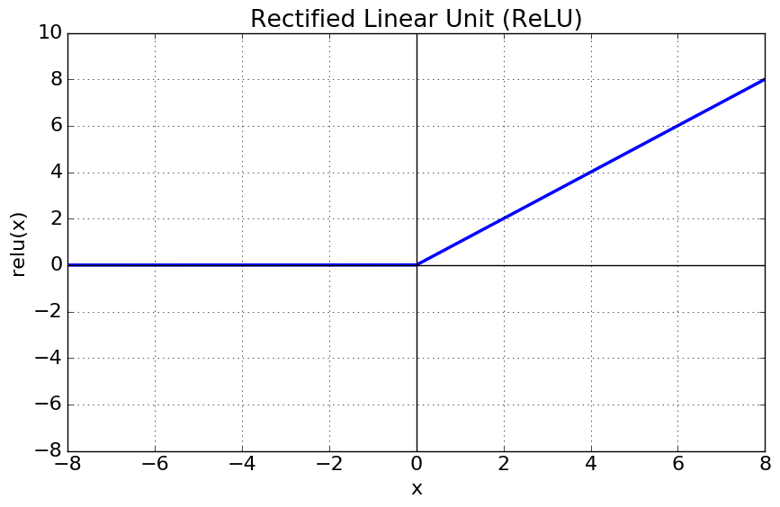
- Features
- It makes the vanishing gradient problem(tanh, sigmoid have) MUCH WORSE,since for all negative values the derivative is precisely zero.
- Computational Cost is not significant.
- In comparison to (sigmoid,tanh), convergence speed is much better.
2. softmax
- Features
- A function that normalizes the output value of a neuron at the last stage for class classification.(normalize sigmoid function)
- So, we can think that It converts the output into probability. (sum = 1.0)
결과에 대한 분석
우선 케라스의 Sequential Model, compile, fit과 activation function에 대해 간략히 적어보았다. 이전에 있어보이려고 영어로 적어봤는데 아까워서 그냥 붙여썼다.
결과에 대해 다뤄보자면, epoch= 20으로 수행한 결과 어느정도까지는 accuracy는 높아지고 loss는 낮아지는 좋은 현상이 일어났지만 그 이후로는 줄어들었다 늘어났다를 반복하여 결론적으로는 성능이 더 낮아졌다. 그 이유는 무엇일까?
정답은 이미지를 벡터로 표현했기 때문이다. 저번 시간에도 말했듯 이미지를 벡터화한다면 조금만 translation되어도 다른 이미지로 인식하므로 overfitting되는 결과가 나온다. 따라서 이를 방지하고자 CNN을 사용하는 것이다.
Convolution을 한 모델로 새롭게 해보자.
New Model with Convolution
새로 들어가기에 앞서 이 서버는 다른분들도 사용하셔서 항상 리소스를 반환해줘야한다.
따라서 학습이 끝난 후 리소스를 반환해주자.
1 | import IPython |
{'status': 'ok', 'restart': True}1 | # using gpu:/1 |
1 | # using gpu:/1 |
1 | from tensorflow.keras.datasets import mnist |
여기까지의 내용은 동일하다.
1 | model = Sequential() |
Model: "sequential_1"
_________________________________________________________________
Layer (type)                 Output Shape              Param #
=================================================================
conv2d_2 (Conv2D)            (None, 26, 26, 64)        640
_________________________________________________________________
conv2d_3 (Conv2D)            (None, 24, 24, 32)        18464
_________________________________________________________________
flatten_1 (Flatten)          (None, 18432)             0
_________________________________________________________________
dense_1 (Dense)              (None, 10)                184330
=================================================================
Total params: 203,434
Trainable params: 203,434
Non-trainable params: 0
_________________________________________________________________
Epoch 1/20
1875/1875 [==============================] - 7s 4ms/step - loss: 0.1776 - accuracy: 0.9570 - val_loss: 0.1147 - val_accuracy: 0.9729
Epoch 2/20
1875/1875 [==============================] - 7s 4ms/step - loss: 0.0854 - accuracy: 0.9766 - val_loss: 0.0864 - val_accuracy: 0.9778
Epoch 3/20
1875/1875 [==============================] - 8s 4ms/step - loss: 0.0745 - accuracy: 0.9797 - val_loss: 0.0905 - val_accuracy: 0.9735
Epoch 4/20
1875/1875 [==============================] - 8s 4ms/step - loss: 0.0724 - accuracy: 0.9802 - val_loss: 0.0919 - val_accuracy: 0.9781
Epoch 5/20
1875/1875 [==============================] - 8s 4ms/step - loss: 0.0700 - accuracy: 0.9812 - val_loss: 0.0837 - val_accuracy: 0.9746
Epoch 6/20
1875/1875 [==============================] - 8s 4ms/step - loss: 0.0690 - accuracy: 0.9818 - val_loss: 0.1036 - val_accuracy: 0.9742
Epoch 7/20
1875/1875 [==============================] - 8s 4ms/step - loss: 0.0690 - accuracy: 0.9818 - val_loss: 0.1009 - val_accuracy: 0.9750
Epoch 8/20
1875/1875 [==============================] - 7s 4ms/step - loss: 0.0689 - accuracy: 0.9819 - val_loss: 0.1134 - val_accuracy: 0.9746
Epoch 9/20
1875/1875 [==============================] - 8s 4ms/step - loss: 0.0700 - accuracy: 0.9819 - val_loss: 0.1004 - val_accuracy: 0.9760
Epoch 10/20
1875/1875 [==============================] - 8s 4ms/step - loss: 0.0692 - accuracy: 0.9826 - val_loss: 0.1298 - val_accuracy: 0.9750
Epoch 11/20
1875/1875 [==============================] - 8s 4ms/step - loss: 0.0681 - accuracy: 0.9827 - val_loss: 0.1055 - val_accuracy: 0.9732
Epoch 12/20
1875/1875 [==============================] - 7s 4ms/step - loss: 0.0688 - accuracy: 0.9820 - val_loss: 0.1205 - val_accuracy: 0.9725
Epoch 13/20
1875/1875 [==============================] - 7s 4ms/step - loss: 0.0682 - accuracy: 0.9830 - val_loss: 0.1140 - val_accuracy: 0.9751
Epoch 14/20
1875/1875 [==============================] - 8s 4ms/step - loss: 0.0671 - accuracy: 0.9830 - val_loss: 0.1266 - val_accuracy: 0.9729
Epoch 15/20
1875/1875 [==============================] - 8s 4ms/step - loss: 0.0664 - accuracy: 0.9831 - val_loss: 0.1417 - val_accuracy: 0.9723
Epoch 16/20
1875/1875 [==============================] - 7s 4ms/step - loss: 0.0639 - accuracy: 0.9837 - val_loss: 0.1319 - val_accuracy: 0.9729
Epoch 17/20
1875/1875 [==============================] - 8s 4ms/step - loss: 0.0670 - accuracy: 0.9837 - val_loss: 0.1290 - val_accuracy: 0.9723
Epoch 18/20
1875/1875 [==============================] - 7s 4ms/step - loss: 0.0668 - accuracy: 0.9840 - val_loss: 0.1517 - val_accuracy: 0.9736
Epoch 19/20
1875/1875 [==============================] - 7s 4ms/step - loss: 0.0625 - accuracy: 0.9849 - val_loss: 0.1545 - val_accuracy: 0.9699
Epoch 20/20
1875/1875 [==============================] - 7s 4ms/step - loss: 0.0640 - accuracy: 0.9845 - val_loss: 0.1448 - val_accuracy: 0.9691
epoch를 20으로 했더니 train data들은 대부분 loss도 감소하고 accuracy도 증가하지만
test data들은 loss도 들쭉날쭉에 accuracy는 감소하기까지한다.
아직 overfitting의 문제를 해결하지 못했을 뿐만아니라 vanishing/exploding gradient또한 해결하지 못했다.
이는 다음 실습에서 batchnormalization과 dropdout에 대해 공부해보고 좀 더 지켜보도록 하겠다.
1 | n = 90 |
랜덤하게 추출해서 확인해보자.
1 | np.random.seed(0) |
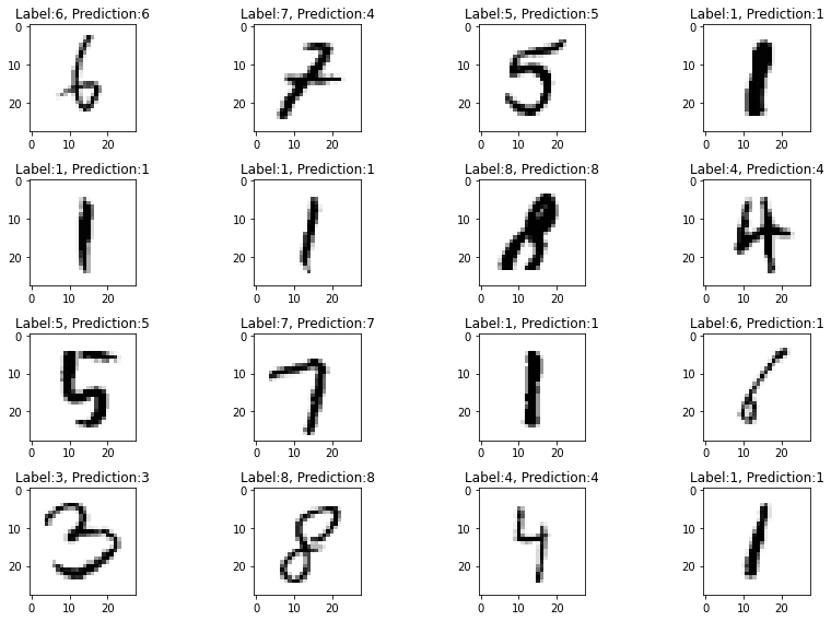
약간의 오차가 있는 듯하다. 이는 다른 Layer들을 공부하면서 줄여보도록 하겠다.
그리고 리소스반환도 필수다!
1 | import IPython |
{'status': 'ok', 'restart': True}